Missing Value Analysis - R

We are going to do missing value analysis on a dataset. Its going to be full of R commands.

Load Required Libraries

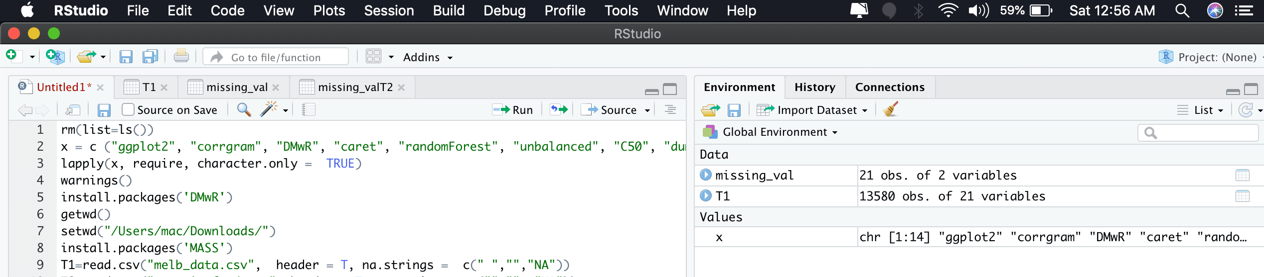
x = c (“ggplot2”, “corrgram”, “DMwR”, “caret”, “randomForest”, “unbalanced”, “C50”, “dummies”, “e1071”, “Information”, “MASS”, “rpart”, “gbm”, “ROSE”)

Note :- DMwR - This library is required for KNN imputation

Set Working Directory

setwd(“/Users/mac/Downloads/“)

Read Data

T1=read.csv(“melb_data.csv”, header = T, na.strings = c(” ”,"",“NA”))
Note:- na.strings- The na.strings parameter of the read function can be used to tell R which symbols/characters need to be treated as NA values

Screenshot for above commands

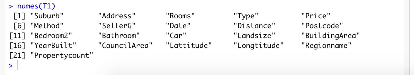
List the column names

names(T1)

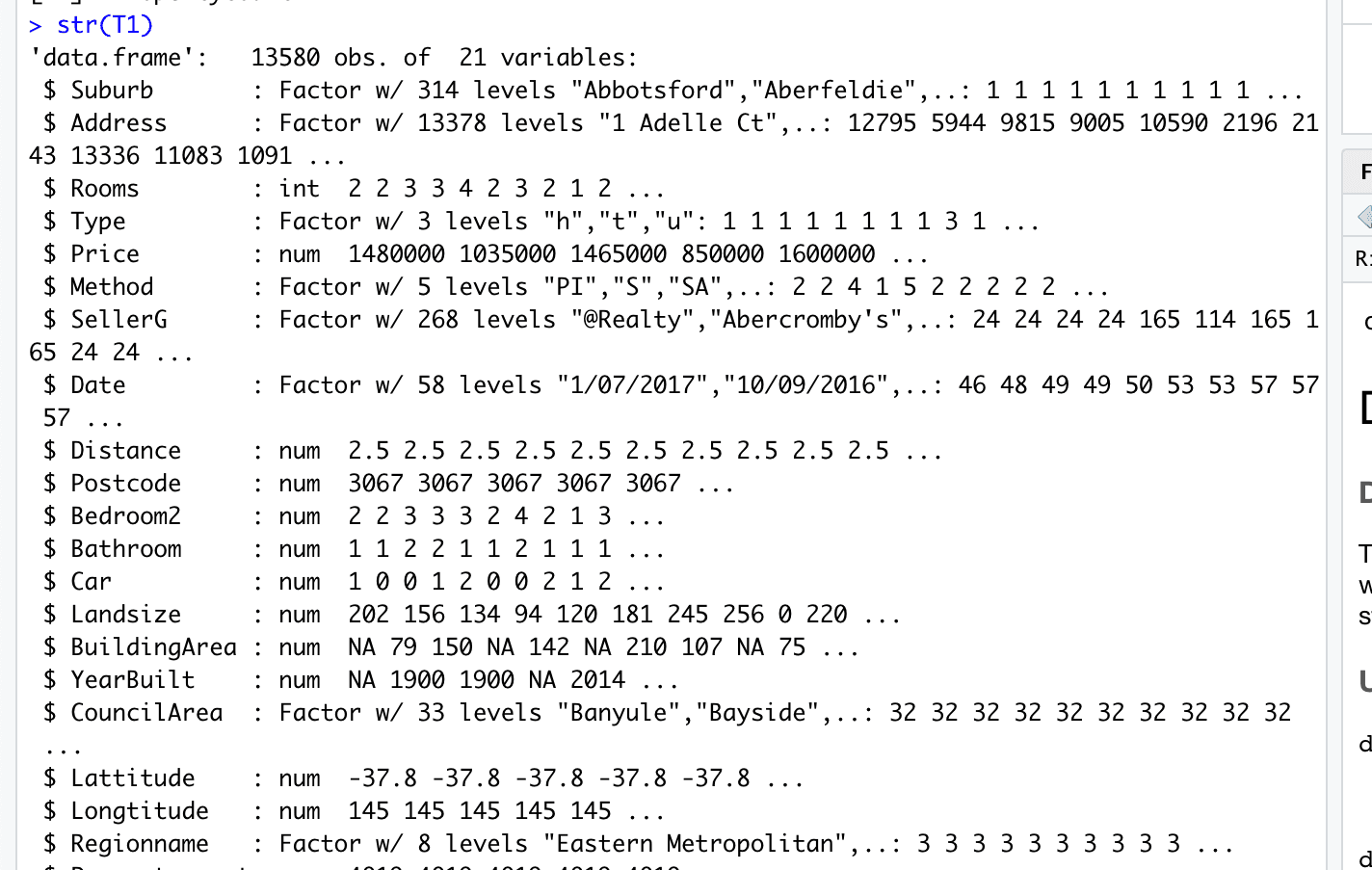
Explore the data

str(T1)

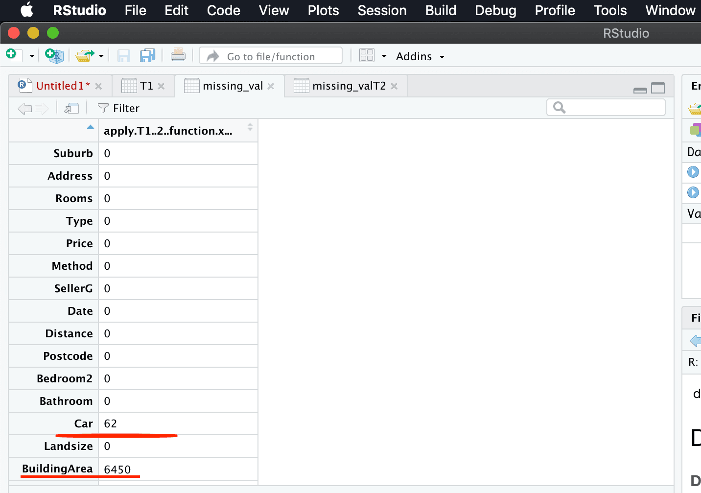
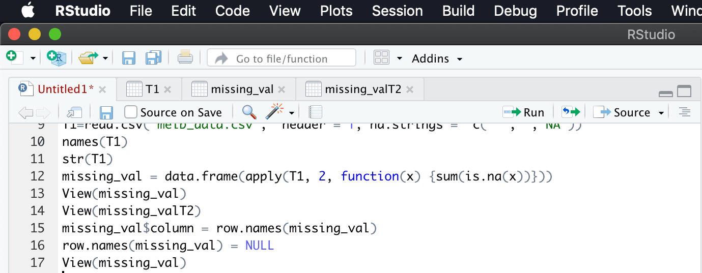
Create Dataframe with total number of missing values

missing_val = data.frame(apply(T1, 2, function(x) {sum(is.na(x))}))
We calculate total number of missing values for every column
Here we use apply function to avoid loop
Inside apply, we pass the arguments like T1, and 2( since we do column level operation), and we create our own function named function, which calculates the number of missing values.

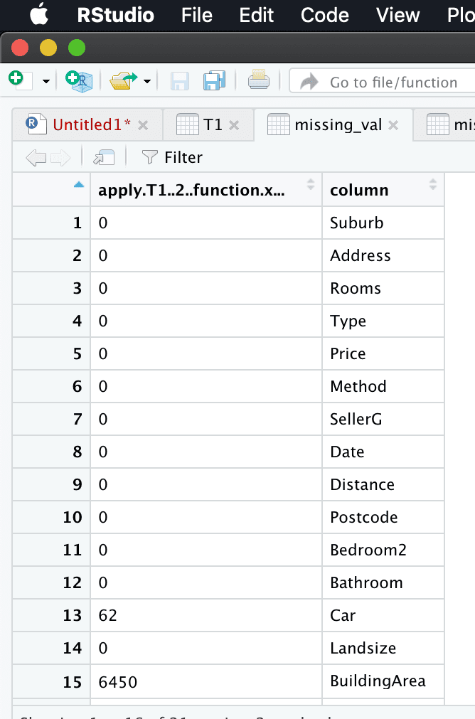
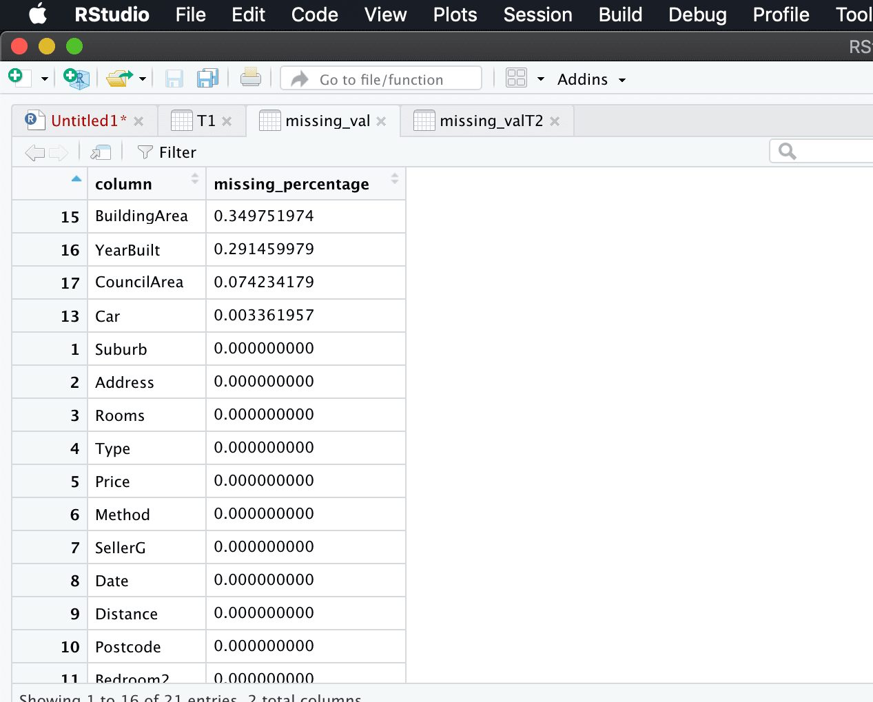
Viewing the dataframe created

View(missing_val)

Convert row names into column

missingval$columns = row.names(missingval)//Adding row names into a separate column
row.names(missing_val) = NULL // Null row.names.

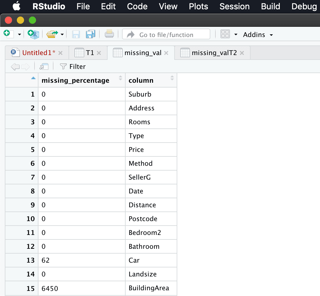
Rename the column

names(missingval)[1] = “missingpercentage” // Rename the first column as missing percentage

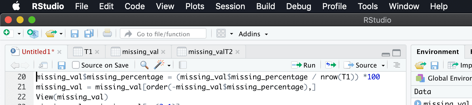
Calculate percentage

missingval$missingpercentage = (missingval$missingpercentage / nrow(T1)) *100

Arrange in descending order

missingval = missingval[order(-missingval$missingpercentage),]

View in ascending order after percentage calculation

View(missing_val)

Rearranging the columns

missingval = missingval[,c(2,1)]

write the output results back into the disk

write.csv(missingval, “Missingperc.csv”, row.names = F)

Below are three methods of missing value analysis. Now, take one value and remove it manually and impute all three methods and identify which method value gets closer to actual value and fix the method for analysis.

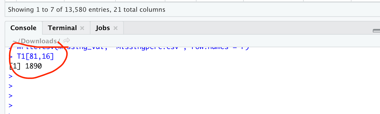
Now I am checking “YearBuilt” variable, 81th row and 16th column. and the answer is below.

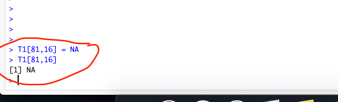
Now i am manually making it as NA and going to compute all three methods

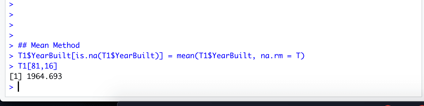
Mean Method

T1$YearBuilt[is.na(T1$YearBuilt)] = mean(T1$YearBuilt, na.rm = T)

Refresh the data before proceeding to next method.

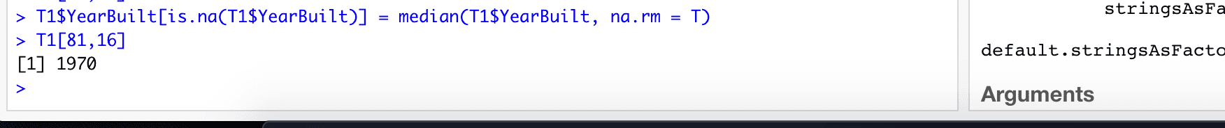
Median Method

T1$YearBuilt[is.na(T1$YearBuilt)] = median(T1$YearBuilt, na.rm = T)

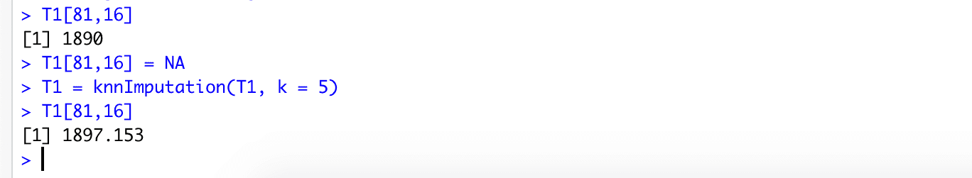
KNN Imputation

T1 = knnImputation(T1, k = 5)
If you get an error, couldnot find Knn function please install library “DMwR”
library(“DMwR”)

Now the actual value of 81st row and 16th column of yearbuilt variable
Actual Value = 1890
We made this value NA and calculated below values
Using Mean the value is = 1964
Using Median the value is = 1970
Using KNN the value is = 1897

And the nearest value is 1897, so we go with KNN method for calculating all missing values.

Hope this post helps! will update you all with next post soon!!!